Intraspecific variation in the thermal tolerance of microscopic giant kelp (Macrocystis pyrifera) sporophytes was tested using a common garden experiment, where 49 unique family-lines were raised under four different water temperatures (12, 16, 20, and 24°C). The unique family-lines were taken from ongoing giant kelp gametophyte cultures held at IMAS, and represented F1 offspring from seven 'selfed' individuals collected from 6 sites across ~250km in Tasmania, Australia, in addition to a site-level cross from each of the sites, and a panmictic cross using the 42 pure family lines. Survivorship of the selected warm-adapted family-lines after outplanting trials at restoration sites can be found here with the associated dataset "NESP Marine Hub Project E7 outplanted kelp survivorship". https://metadata.imas.utas.edu.au/geonetwork/srv/eng/catalog.search#/metadata/908afd8c-cc7a-4ea3-a87e-4497ae8da87a

The spatial extent of C. rodgersii "barrens" was estimated by surveying rocky reef habitat with a towed underwater video system. Sampling took place at 13 regions along the east coast of Tasmania, each comprising 3 subsites, this dataset refers to the Recherche region, and its 3 subsites: Eliza Point, Fisher Point and Actaeons.

Seasonal patterns in the in situ ecophysiology of the common habitat-forming seaweeds Ecklonia radiata, Phyllospora comosa, and Macrocystis pyrifera were investigated at different latitudes and depths in southeastern Australia. We used multiple performance indicators (photosynthetic characteristics, pigment content, chemical composition, stable isotopes, nucleic acids) to assess the ecophysiology of seaweeds near the northern and southern margins of their range, along a depth gradient (E. radiata only), over a two year period (September 2010 – August 2012).

The recruitment of mussels and microphytobenthic (MPB) algae to 28 experimental artificial reefs supporting different patch sizes and density of kelp (Ecklonia radiata) off Maria Island, Tasmania. The recruitment of mussels was assessed using rope fibre habitats, and the recruitment of MPB algae was assessed using microscope slides, positioned across the artificial reef and collected in November 2015. These data were collected to examine how the patch size and density of kelp influences the establishment of MPB algae and mussels.

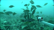
The data is quantitative abundance of fish, megafaunal invertebrates and percent algal cover derived from underwater visual census methods involving transect counts at rocky reef sites around Tasmania. This dataset allows examination of changes in Tasmanian shallow reef faunal and floral communities over a decadal scale, with initial surveys conducted in 1992-1995, and again in 2006-2007. There are plans for ongoing surveys. An additional component was added in the latter study - a boat ramp study looking at the proximity of boat ramps and their effects of fishing. We analysed underwater visual census data on fishes and macroinvertebrates (abalone and rock lobsters) at 133 shallow rocky reef sites around Tasmania that ranged from 0.6 - 131 km from the nearest boat ramp. These sites were not all the same as those used for the comparison of 1994 and 2006 reef communities. The subset of 133 sites examined in this component consisted of only those sites that were characterized by the two major algal (kelp) types (laminarian or fucoid dominated). Sites with atypical algal assemblages were omitted from the 196 sites surveyed in 2006. This study aimed to examine reef community data for changes at the community level, changes in species richness and introduced species populations, and changes that may have resulted from ocean warming and fishing. The methods are described in detail in Edgar and Barrett (1997). Primarily the data are derived from transects at 5 m depth and/or 10 m depth at each site surveyed. The underwater visual census (UVC) methodology used to survey rocky reef communities was designed to maximise detection of (i) changes in population numbers and size-structure (ii) cascading ecosystem effects associated with disturbances such as fishing, (iii) long term change and variability in reef assemblages.

An aerial survey was conducted for giant kelp (Macrocystis pyrifera) on the east coast of Tasmania from Eddystone Point to Southeast Cape. This survey represents part of a series of similar surveys, with historic aerial surveys having been conducted in 1986 and 1999. The survey was conducted via light aircraft. Areas of visable Macrocystis pyrifera beds were marked on topographical land tenure maps using landmarks as references, and complimentary photo footage was collected.

-- Layton et al. Chemical microenvironments within macroalgal assemblages: implications for the inhibition of kelp recruitment by turf algae. Limnology & Oceanography. DOI:10.1002/lno.11138 -- Kelp forests around the world are under increasing pressure from anthropogenic stressors. A widespread consequence is that in many places, complex and highly productive kelp habitats have been replaced by structurally simple and less productive turf algae habitats. Turf algae habitats resist re-establishment of kelp via recruitment inhibition; however little is known about the specific mechanisms involved. One potential factor is the chemical environment within the turf algae and into which kelp propagules settle and develop. Using laboratory trials, we illustrate that the chemical microenvironment (O2 concentration and pH) 0.0–50 mm above the benthos within four multispecies macroalgal assemblages (including a turf-sediment assemblage and an Ecklonia radiata kelp-dominated assemblage) are characterised by elevated O2 and pH relative to the surrounding seawater. Notably however, O2 and pH were significantly higher within turf-sediment assemblages than in kelp-dominated assemblages, and at levels that have previously been demonstrated to impair the photosynthetic or physiological capacity of kelp propagules. Field observations of the experimental assemblages confirmed that recruitment of kelp was significantly lower into treatments with dense turf algae than in the kelp-dominated assemblages. We demonstrate differences between the chemical microenvironments of kelp and turf algae assemblages that correlate with differences in kelp recruitment, highlighting how degradation of kelp habitats might result in the persistence of turf algae habitats and the localised absence of kelp.

Quantitative surveys were undertaken at four sites in the Kent Group, north eastern Tasmania (southern and northern shores of East Cove at Deal Island, Winter Cove at Deal Island, NE coast of Dover Island) by divers using underwater visual census methods to survey the reef habitat.

The National Outfall Database (NOD) project addresses the need of government and community to understand the impacts on health and the ocean environment that occur from sewerage outfalls around Australia. This dataset is part of the assessment and mapping of the marine impacts of wastewater disposal to ocean and estuarine waters in Australia. The data collected in this study is intended to be used to assist decision makers to understand risk and prioritise investment, to help the public understand water and wastewater management and make decisions when choosing recreation locations, and private operators seeking to re-use wastewater or products found within wastewater. Each outfall is divided into three levels of data; one (1) being basic information such as location, treatment, governance and size; two (2) being more detailed information taken from publicly available annual environmental monitoring reports, licence and other information; and three (3) containing highly detailed information such as daily performance data and receiving waters ecosystem assessments and studies to enable researchers and others to undertake comparative studies. The data custodian will make a data report and methodology available to provide a full explanation of this database. The National Outfall Database is an online resource available here: https://www.outfalls.info/ The database currently tracks 48 indicators across 192 monitoring sites. The data is also available for download in CSV format in the "online resources" section of this record, and will continue to be updated as new data becomes available (data currently available to 30/06/2022 - last checked 19/01/2024.